A Bayesian Approach to Basketball

06-01-2020 statistics, tutorial

motivation

Bayesian inference is the process of using evidence (data) to update one’s prior beliefs about phenomena. The Bayesian approach can be especially useful in a field like sports, where we often don’t have large samples to work with (rendering frequentist approaches less effective). In this post, I’ll apply Bayesian principles in a basketball context.

prerequisites

This post assumes that the reader is familiar with probability theory and notation. I’ll provide a quick review, but I recommend reading up on Conditional Probability, Bayes’ Theorem, and the Law of Total Probability.

Conditional Probability

$P (A | B) = \frac{P (A, B)}{P (B)}$ This says that the probability of event $A$ conditioned on event $B$ (we usually say “ $A$ given $B$ ”) is equal to the joint probability of $A$ and $B$ divided by the probability of $B$ .

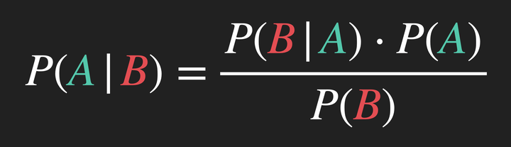
Bayes’ Theorem

Bayesian inference is centered around one equation: Bayes’ Theorem. $P (H | E) = \frac{P (E | H) \cdot P (H)}{P (E)}$ Here’s a quick summary of the various parts of the theorem:

$H$ represents the hypothesis, which is updated based on $E$ , the evidence.
$P (H)$ is called the prior probability. This is the probability of $H$ prior to observing $E$ .
$P (E | H)$ is called the likelihood. This is the probablity of observing $E$ given that $H$ is true.
$P (E)$ is the total probability of the evidence being observed, we’ll use the Law of Total Probability to break this out. According to Wikipedia, $P (E)$ is sometimes called the marginal likelihood.
$P (H | E)$ is the posterior probability. The is the probability of $H$ given that we have observed $E$ . In simpler terms, this is the updated probability of our hypothesis after we’ve accounted for new evidence.

Law of Total Probability

$P (A) = \sum_{i = 1}^{n} P (A, B_{i})$ The Law of Total Probability just says that the total probability of some event, $A$ , is equal to the sum of the joint probabilities of $A$ and all other disjoint sets, $B_{i}$ , in the probability space.

bayesian inference applied to basketball

problem

Suppose a good 3-point shooter makes 35% of their 3-pointers from the top of the arc, and a bad one makes 15% of their 3-pointers from the top of the arc.

We want to know if Christina is a good 3-point shooter. Before she shoots, we think that there is a 20% chance of her being a good 3-point shooter. Christina takes three 3-point shots from the top of the arc, and makes all three.

What is the probability that Christina is a good 3-point shooter?
How many 3-point shots from the top of the arc would Christina have to make in a row for us to believe there’s at least a 95% chance Christina is a good 3-point shooter?

solution

> part 1.

Based on the problem statement, we want to update our belief about Christina being a good 3-point shooter for each shot that she makes in a row. So, $H$ – our hypothesis – is that Christina is a good 3-point shooter, and $E$ – the evidence – is that she makes three shots in a row. Since we’re going to update our prior probability iteratively, I’m going to modify our notation a bit, and define $E_{i}$ as the $i$ th shot that she makes in a row (i.e. $E_{1}$ is the first make, $E_{2}$ is the second make, etc.),

From the problem statement:

$P (H) = 0.20 ⟺ P (\neg H) = 0.80$
$P (E_{i} | H) = 0.35$
$P (E_{i} | \neg H) = 0.15$
$P (E_{i}) = P (E_{i}, H) + P (E_{i}, \neg H) = P (E_{i} | H) \cdot P (H) + P (E_{i} | \neg H) \cdot P (\neg H)$ (by the Law of Total Probability)

Let’s look at our Bayesian update after Christina makes her first shot: $\begin{aligned} P (H | E_{1}) & = \frac{P (E_{1} | H) \cdot P (H)}{P (E_{1})} \\ = \frac{P (E_{1} | H) \cdot P (H)}{P (E_{1} | H) \cdot P (H) + P (E_{1} | \neg H) \cdot P (\neg H)} \\ = \frac{0.35 \cdot 0.20}{0.35 \cdot 0.20 + 0.15 \cdot 0.80} \end{aligned}$

Here’s our posterior probability after Christina makes her first shot: $P (H | E_{1}) =$ 0.3684211.
We can now update our prior probability: $P (H) := P (H | E_{1})$ .

We can apply the same iterative update procedure to find the posterior probabilities after Christina’s second and third made shots, but first, let’s see if we can simplify our equation a bit. We’ll start by examining the equation for the posterior after Christina’s second make: $\begin{aligned} P (H | E_{2}) & = \frac{P (E_{2} | H) \cdot P (H)}{P (E_{2})} \\ = \frac{P (E_{2} | H) \cdot P (H)}{P (E_{2} | H) \cdot P (H) + P (E_{2} | \neg H) \cdot P (\neg H)} \end{aligned}$ Now, remember, we updated our initial prior probability: ( $P (H) := P (H | E_{1})$ and $P (\neg H) := 1 - P (H | E_{1})$ ).
So: $\begin{aligned} P (H | E_{2}) & = \frac{P (E_{2} | H) \cdot P (H | E_{1})}{P (E_{2} | H) \cdot P (H | E_{1}) + P (E_{2} | \neg H) \cdot P (\neg H | E_{1})} \\ = \frac{P (E_{2} | H) \cdot \frac{P (E_{1} | H) \cdot P (H)}{P (E_{1} | H) \cdot P (H) + P (E_{1} | \neg H) \cdot P (\neg H)}}{P (E_{2} | H) \cdot \frac{P (E_{1} | H) \cdot P (H)}{P (E_{1} | H) \cdot P (H) + P (E_{1} | \neg H) \cdot P (\neg H)} + P (E_{2} | \neg H) \cdot (1 - \frac{P (E_{1} | H) \cdot P (H)}{P (E_{1} | H) \cdot P (H) + P (E_{1} | \neg H) \cdot P (\neg H)})} \end{aligned}$ We can simplify this further by noting that $1 - \frac{P (E_{1} | H) \cdot P (H)}{P (E_{1} | H) \cdot P (H) + P (E_{1} | \neg H) \cdot P (\neg H)} = \frac{P (E_{1} | \neg H) \cdot P (\neg H)}{P (E_{1} | H) \cdot P (H) + P (E_{1} | \neg H) \cdot P (\neg H)}$ .
Now, we have: $\begin{aligned} P (H | E_{2}) & = \frac{P (E_{2} | H) \cdot \frac{P (E_{1} | H) \cdot P (H)}{P (E_{1} | H) \cdot P (H) + P (E_{1} | \neg H) \cdot P (\neg H)}}{P (E_{2} | H) \cdot \frac{P (E_{1} | H) \cdot P (H)}{P (E_{1} | H) \cdot P (H) + P (E_{1} | \neg H) \cdot P (\neg H)} + P (E_{2} | \neg H) \cdot \frac{P (E_{1} | \neg H) \cdot P (\neg H)}{P (E_{1} | H) \cdot P (H) + P (E_{1} | \neg H) \cdot P (\neg H)}} \\ = \frac{P (E_{2} | H) \cdot P (E_{1} | H) \cdot P (H)}{P (E_{2} | H) \cdot P (E_{1} | H) \cdot P (H) + P (E_{2} | \neg H) \cdot P (E_{1} | \neg H) \cdot P (\neg H)} \end{aligned}$ I won’t write out all of the math, but if you follow the same procedure to find the posterior probability after Christina’s third made shot, you’ll get the following: $\begin{aligned} P (H | E_{3}) & = \frac{P (E_{3} | H) \cdot P (E_{2} | H) \cdot P (E_{1} | H) \cdot P (H)}{P (E_{3} | H) \cdot P (E_{2} | H) \cdot P (E_{1} | H) \cdot P (H) + P (E_{3} | \neg H) \cdot P (E_{2} | \neg H) \cdot P (E_{1} | \neg H) \cdot P (\neg H)} \end{aligned}$ Do you see the pattern? Let me make it a bit more obvious. In the following equation, $P (H | E_{n})$ represents the posterior probability of Christina being a good 3-point shooter, given that she has made $n$ shots in a row from the top of the arc. $\begin{aligned} P (H | E_{n}) & = \frac{[\prod_{i = 1}^{n} P (E_{i} | H)] \cdot P (H)}{[\prod_{i = 1}^{n} P (E_{i} | H)] \cdot P (H) + [\prod_{i = 1}^{n} P (E_{i} | \neg H)] \cdot P (\neg H)} \end{aligned}$ But the probability of making a shot from the top of the arc given that you’re a good or bad shooter doesn’t change. As we noted earlier, $P (E_{i} | H) = 0.35$ and $P (E_{i} | \neg H) = 0.15$ , regardless of the shot number ( $i$ ). This is another way of saying that $E_{1} | H, E_{2} | H, \dots, E_{n} | H$ are conditionally independent and identical ( $E_{1} | \neg H, E_{2} | \neg H, \dots, E_{n} | \neg H$ are conditionally independent and identical as well). These properties allow us to make a final simplification: $\begin{aligned} P (H | E_{n}) & = \frac{[P (E_{1} | H) \cdot P (E_{2} | H) \cdot . . . \cdot P (E_{n} | H)] \cdot P (H)}{[P (E_{1} | H) \cdot P (E_{2} | H) \cdot . . . \cdot P (E_{n} | H)] \cdot P (H) + [P (E_{1} | \neg H) \cdot P (E_{2} | \neg H) \cdot . . . \cdot P (E_{n} | \neg H)] \cdot P (\neg H)} \\ = \frac{[P (E_{i} | H)]^{n} \cdot P (H)}{[P (E_{i} | H)]^{n} \cdot P (H) + [P (E_{i} | \neg H)]^{n} \cdot P (\neg H)} \end{aligned}$ It took some work, but we finally have a simple equation for calculating the posterior after $n$ made shots. Let’s finish up part 1 of the problem: $\begin{aligned} P (H | E_{3}) & = \frac{[P (E_{i} | H)]^{3} \cdot P (H)}{[P (E_{i} | H)]^{3} \cdot P (H) + [P (E_{i} | \neg H)]^{3} \cdot P (\neg H)} \\ = \frac{(0.35)^{3} \cdot 0.20}{(0.35)^{3} \cdot 0.20 + (0.15)^{3} \cdot 0.80} \end{aligned}$

The posterior probability after Christina makes her third shot in a row: $P (H | E_{3}) =$ 0.7605322.

> part 2.

We can write a simple loop to figure out how many makes in a row it would take for us to believe there’s at least a 95% chance Christina is a good 3-point shooter:

# clear environment
rm(list=ls())

# variables
p_h <- 0.2  # prior probability
p_e_given_h <- 0.35  # probability of making shot given good shooter
p_e_given_not_h <- 0.15  # probability of making shot given bad shooter

posterior <- 0
thresh <- 0.95
i <- 0

# loop through shots until threshold is breached
while (posterior < thresh) {
  # update shot iteration
  i <- i + 1
  # find posterior probability and update the prior
  posterior <- (p_e_given_h^i * p_h) / (p_e_given_h^i * p_h + p_e_given_not_h^i * (1-p_h))
  
  bayes_update <- glue::glue(
    "shots made in a row: {i} \nposterior probability: {posterior}\n\n"
  )
  print(bayes_update)
}

## shots made in a row: 1 
## posterior probability: 0.368421052631579
## 
## shots made in a row: 2 
## posterior probability: 0.576470588235294
## 
## shots made in a row: 3 
## posterior probability: 0.760532150776053
## 
## shots made in a row: 4 
## posterior probability: 0.881100917431193
## 
## shots made in a row: 5 
## posterior probability: 0.945328758647843
## 
## shots made in a row: 6 
## posterior probability: 0.975813876332269

Christina would have to make 6 shots in a row from the top of the arc for us to believe that there’s a 95% chance at minimum that she is a good 3-point shooter.

> an alternate approach

Let’s try tackling this problem from a different perspective. We’ll start by asking “what’s the probability that a good shooter will make $n$ shots from the top of the arc in a row?” $\begin{aligned} P (E_{1}, \dots, E_{n} | H) & = \frac{P (E_{1}, \dots, E_{n}, H)}{P (H)} \end{aligned}$ But our equation doesn’t include the value that the problem is asking for, $P (H | E_{1}, \dots, E_{n})$ . We can fix this by applying the definition of conditional probability to the term in the numerator.
We then have: $\begin{aligned} P (E_{1}, \dots, E_{n} | H) & = \frac{P (H | E_{1}, \dots, E_{n}) \cdot P (E_{1}, \dots, E_{n})}{P (H)} \end{aligned}$ Now that we’ve got the term of interest in our equation, we can rearrange our equation to isolate it: $\begin{aligned} P (H | E_{1}, \dots, E_{n}) & = \frac{P (E_{1}, \dots, E_{n} | H) \cdot P (H)}{P (E_{1}, \dots, E_{n})} \end{aligned}$ We can break out the denominator using the Law of Total Probability and the definition of conditional probability: $\begin{aligned} P (H | E_{1}, \dots, E_{n}) & = \frac{P (E_{1}, \dots, E_{n} | H) \cdot P (H)}{P (E_{1}, \dots, E_{n}, H) + P (E_{1}, \dots, E_{n}, \neg H)} \\ = \frac{P (E_{1}, \dots, E_{n} | H) \cdot P (H)}{P (E_{1}, \dots, E_{n} | H) \cdot P (H) + P (E_{1}, \dots, E_{n} | \neg H) \cdot P (\neg H)} \end{aligned}$ We can apply the fact that $E_{1} | H ⊥ ⊥ E_{2} | H ⊥ ⊥ \dots ⊥ ⊥ E_{n} | H$ ( $⊥ ⊥$ is just notation for independence) to simplify further: $\begin{aligned} P (H | E_{1}, \dots, E_{n}) & = \frac{P (E_{1} | H) \cdot . . . \cdot P (E_{n} | H) \cdot P (H)}{P (E_{1} | H) \cdot . . . \cdot P (E_{n} | H) \cdot P (H) + P (E_{1} | \neg H) \cdot . . . \cdot P (E_{n} | \neg H) \cdot P (\neg H)} \end{aligned}$ And lastly, we use the facts that $P (E_{i} | H) = P (E_{j} | H) \forall i, j$ and $P (E_{k} | \neg H) = P (E_{l} | \neg H) \forall k, l$ to make a final simplification: $\begin{aligned} P (H | E_{1}, \dots, E_{n}) & = \frac{[P (E_{i} | H)]^{n} \cdot P (H)}{[P (E_{i} | H)]^{n} \cdot P (H) + [P (E_{i} | \neg H)]^{n} \cdot P (\neg H)} \end{aligned}$ We’ve found the same result as when we used the Bayesian update procedure!

wrapping things up

In this post, we worked through a problem dealing with probability in a sports context using two different methods, and we saw that both methods resulted in the same answer. That’s the beauty of math – there’s rarely ever one sole path to the solution. This was meant to be a straightforward use of Bayesian inference to solve a simple problem, but resulted in a pretty lengthy post. For those of you who stuck it out with me, I hope you were able to follow along and that you found the process of solving this problem as rewarding as I did. Thanks for reading!

probability bayesian r