Goal Control: A Tracking-Based Metric for Modelling xG
introduction
Inspired by the Friends of Tracking masterclasses on pitch control and expected goals (xG) given by William Spearman, Laurie Shaw, and David Sumpter I used tracking data to create a metric called goal control that accounts for player positioning in goal-scoring opportunities. In this post, I’ll use this metric to analyze a scoring sequence by Liverpool from 2019. For further details about the computation of goal control, refer to the Appendix included later in this post.
setup
In this analysis, I’ll be focusing on a goal scored by Liverpool against the Wolverhampton Wanderers (Wolves). I took the data provided by Last Row and augmented it with additional variables like velocities (m/s), event identifiers, etc. Here’s a quick sample:
| frame | team | player | player_num | player_role | player_action | x | y | vx | vy |
|---|---|---|---|---|---|---|---|---|---|
| 11 | defense | 3411 | NA | off-ball | NA | 67.84042 | 46.14833 | 0.07177057 | -2.8663321 |
| 25 | defense | 6672 | NA | off-ball | NA | 84.18373 | 40.54557 | 1.36195636 | -1.8817277 |
| 39 | attack | 7621 | NA | off-ball | NA | 74.62945 | 64.50325 | 2.54430104 | -1.9158884 |
| 44 | attack | 1209 | 5 | off-ball | NA | 83.11582 | 48.74664 | 1.65594214 | -2.8149772 |
| 57 | defense | 6671 | NA | off-ball | NA | 86.78585 | 26.68970 | 2.05350559 | -4.1245470 |
| 62 | defense | 6673 | NA | off-ball | NA | 87.13803 | 42.77741 | 2.41616417 | -2.4874652 |
| 78 | defense | 7420 | NA | keeper | NA | 105.19367 | 34.58961 | 1.82586258 | 0.1657452 |
| 100 | defense | 6670 | NA | off-ball | NA | 88.95819 | 17.21975 | 4.37971308 | 2.2846900 |
| 109 | attack | 12 | 66 | passer | NA | 98.02335 | 11.58348 | 6.85120598 | -1.2644982 |
| 132 | defense | 7420 | NA | keeper | NA | 105.64907 | 34.05649 | 0.61289653 | 2.3577691 |
brief intro to goal control
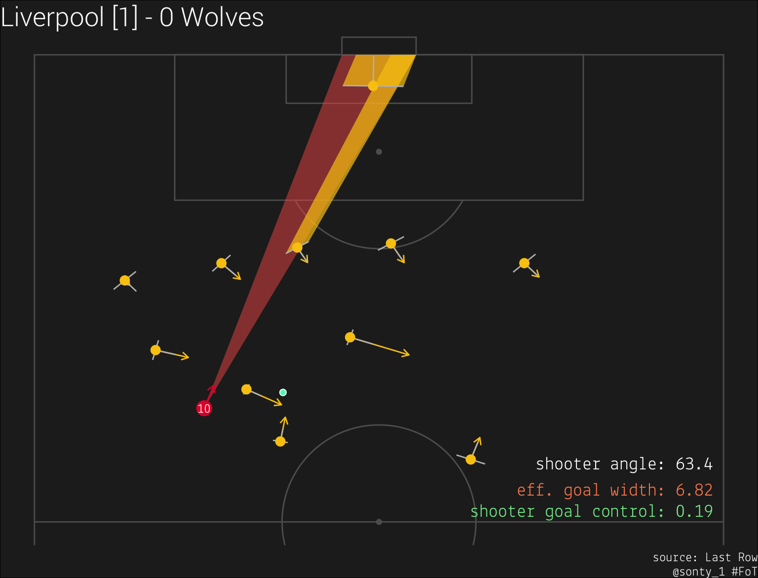
Goal control, denoted \(\Gamma\), aims to quantify the amount of the goal’s width that is controlled by a player or team. Goal control values are always in \([0,1]\), with larger values indicating a higher degree of control. Here’s an example from a frame of Liverpool’s scoring sequence against the Wolves (Liverpool players are red, Wolves players are yellow, and the ball is green):
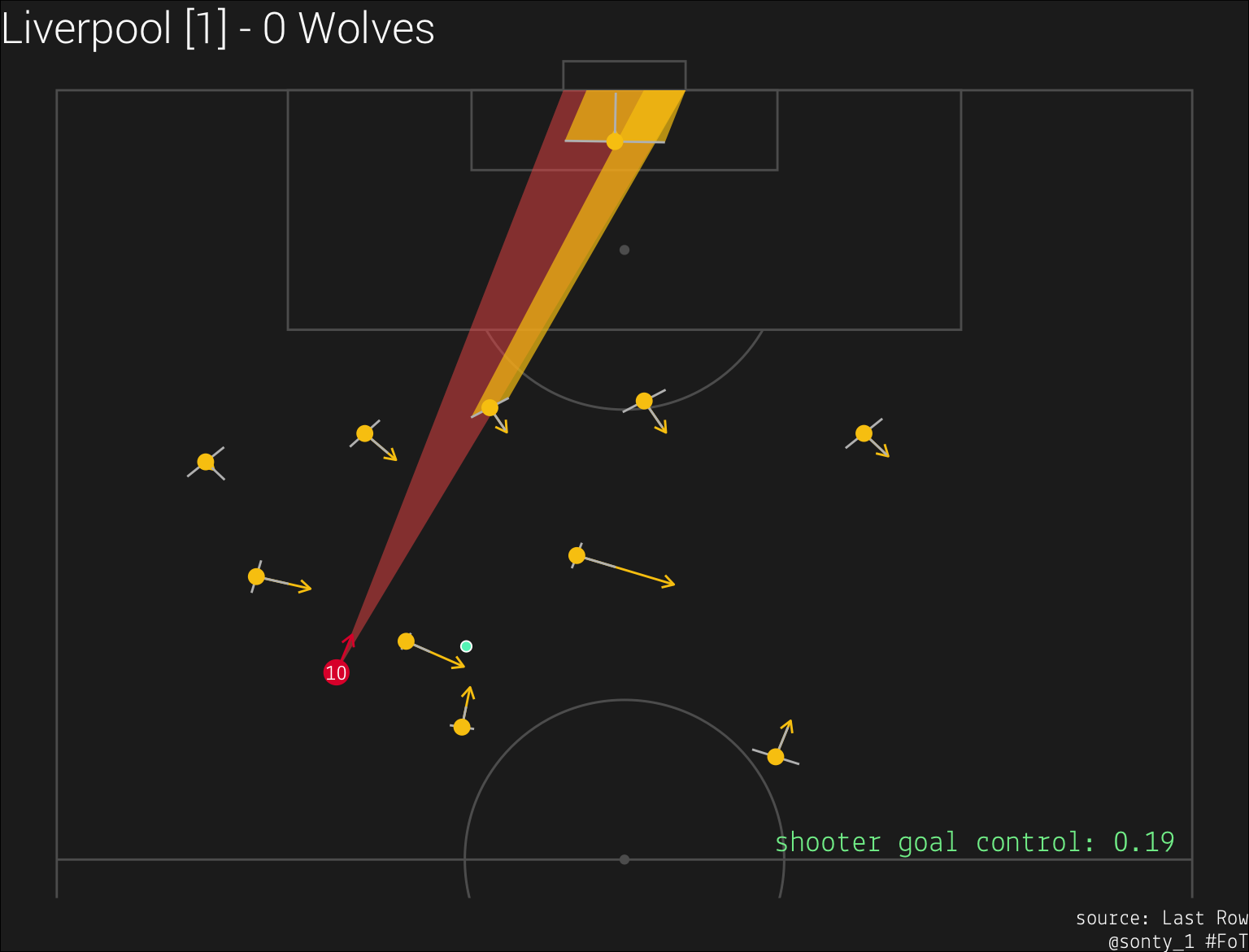 From the above image, we can see that at this moment, Liverpool’s shooter (Sadio Mane, #10) has a goal control value of
 0.19. This means that the two Wolves players that are obstructing Mane’s view of the goal have a combined goal control value of .81.
analysis
For this analysis, I’d like to look at the moments just before the goal was scored. I’ll start by showing the play at half-speed.
From the clip, we can see that one of the Wolves defenders cuts all-the-way across #10’s goal-view, and at one point completely blocks his view on goal. From this point forward, I’ll refer to that Wolves player as “Defender 1”, and highlight him in blue.
Let’s take a look at the moments surrounding the crossing ball delivered by Liverpool’s #66 (Trent Alexander-Arnold):
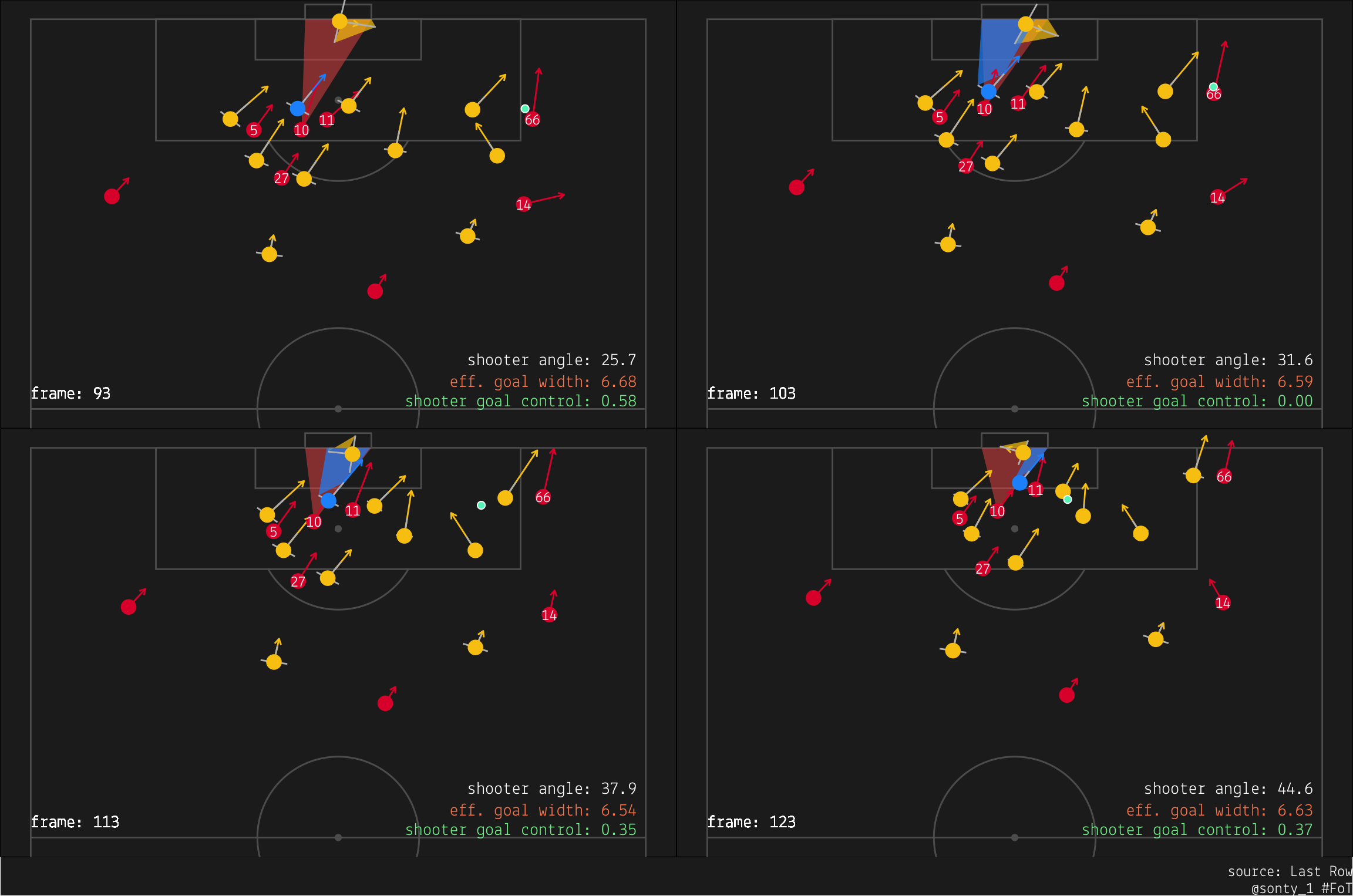
We see that as #66 is advancing the ball, Defender 1 cuts across #10, resulting in #10 momentarily having no goal control. However, #10 begins to slow down, causing Defender 1 to continue moving across his path and shift focus to tracking #11 (Mo Salah) instead. #66, aware of Defender 1’s committal to shadowing #11, crosses the ball to #10, who is slightly further back but now has a much more open view on goal.
Next, let’s examine the moment #10 takes his shot:
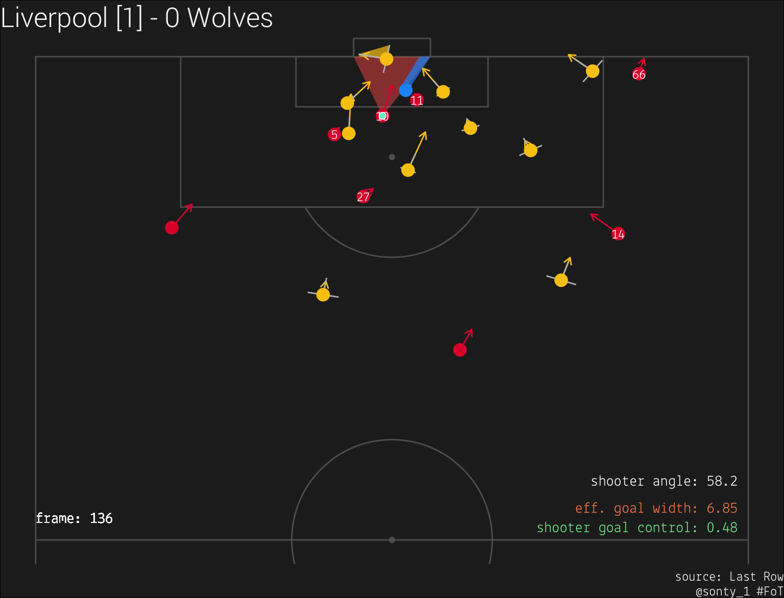
We see that when #10 finally shoots the ball, he has almost half of the goal open to him, and the keeper’s velocity towards the left is opening the goal up even further.
Finally, we can visualize goal control as a time series:
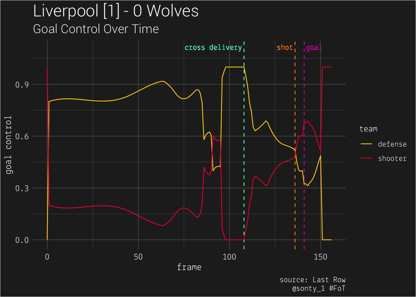 At the moment when #66 crosses the ball to #10, #10 is completely blocked from the goal! However, #10’s goal control steeply increases as soon as the ball is played his way, nears 0.5 as he shoots, and increases even further before the ball crosses the goal-line. #66’s pitch-awareness is downright Promethean – when he has the ball on the wing, it is imperative that the defense accounts for all attackers making runs, not just those who are furthest forward.
conclusion
Liverpool forwards vary their velocities in forward runs not only to create space on the pitch, but also to control more area in the opposition’s goal. Much has already been said about Trent Alexander-Arnold’s prowess in delivering crosses, but what I find even more compelling is his foresight and ability to pick out the attacker that will have the best view on goal, even if he has to send the ball through traffic.
goal control provides a metric that quantifies how “open” the goal is for an attacker, and allows us to visualize how attackers and defenders use positioning to impact goal scoring opportunity. With a larger dataset, goal control could be used to formulate a more accurate xG model. In the future, I’d like to apply this concept to 2-dimensions (i.e. the entire 2-D goal surface, rather than just the 1-D goal line).
one final visualization
I couldn’t resist…
appendix
In this section, I’ll describe the 3 metrics that I displayed in my visuals.
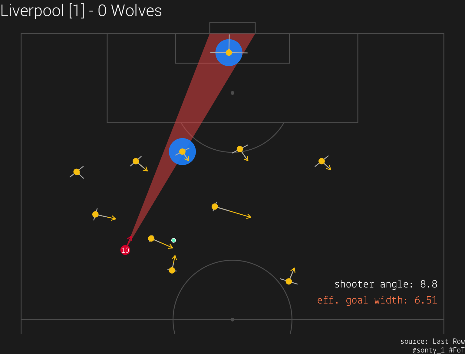
metric 1: shooter angle
This metric has already been detailed in David Sumpter’s book, Soccermatics. Shooter angle is the angle that the shooter has on the opponent’s goal: a larger angle has a strong correlation with higher xG. Since we have two vectors (the vectors from the shooter to the left and right goalposts, \(v_l\) and \(v_r\), respectively), we can compute the shooter angle (\(\theta\)) using the definition of the dot product: \[\theta = cos^{-1}(\frac{v_l \cdot v_r}{|v_l||v_r|})\]
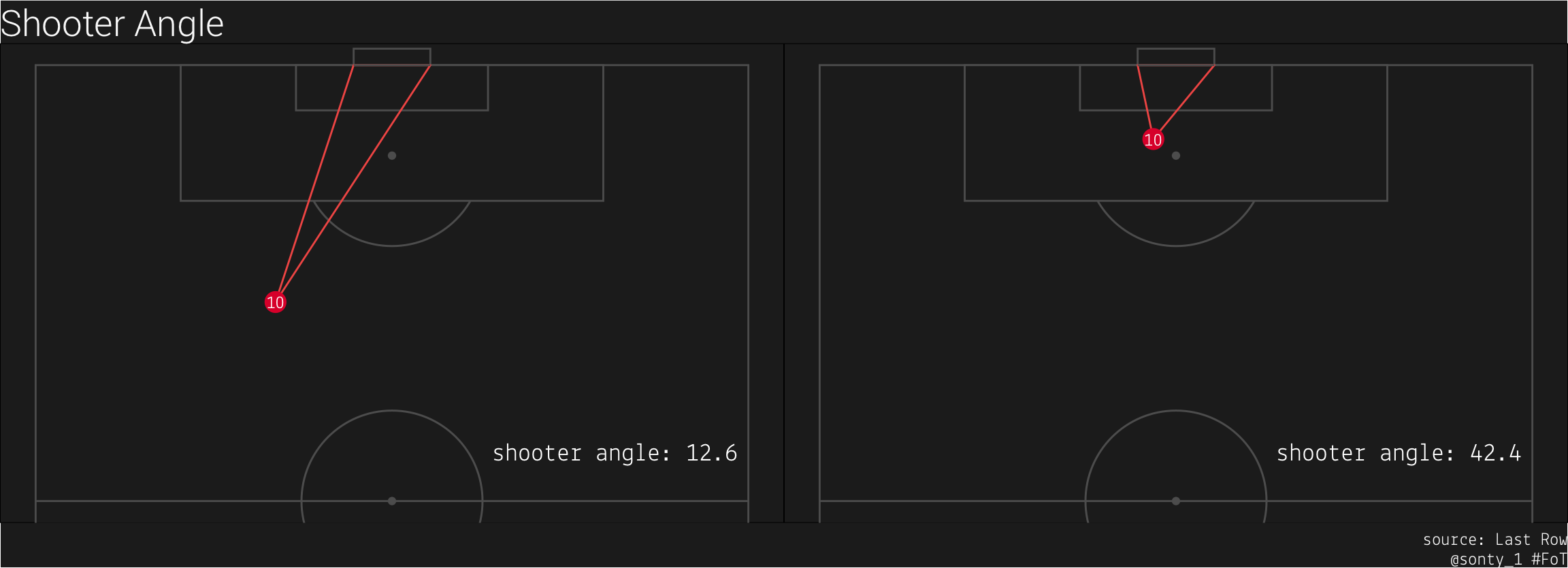
From the above plots, we can see that as the shooter moves closer and more central to the goal, the shooter angle increases.
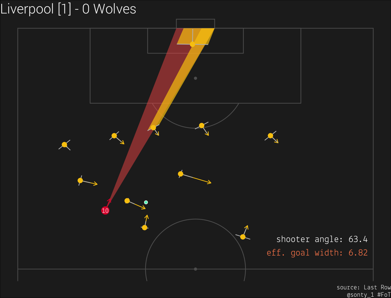
metric 2: effective goal width
This is just an offshoot of shooter angle: the primary reason that xG increases as the shooter moves towards the center of the goal is that they have more goal real estate to attack. Since we have two vectors (the vectors from the shooter to the left and right goalposts, \(v_l\) and \(v_r\), respectively) and the shooter angle \(\theta\), we can compute the effective goal width (\(\omega\)) using \(\theta\) and the shorter of the two vectors, say \(v_s\): \[\omega = 2|v_s|sin(\frac{\theta}{2})\]
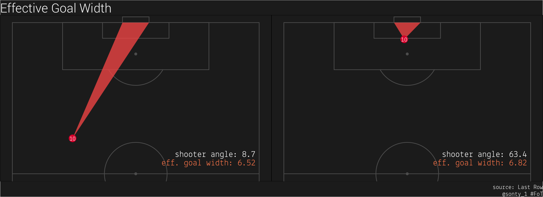
In the plot on the left, 6.52 meters of the goal are available to the shooter, and in the plot on the right, the shooter has 6.82 meters open to him. We could scale the effective goal width to account for the shooter’s distance from the goal, but the shooter angle already encodes that information. I like displaying the effective goal width because I find it easier to intuit a distance than an angle.
metric 3: goal control
It’s clear that angles play a huge role in the success of a shot, so it follows that defenders can use positioning to close off angles (reducing the effective goal width) and severely impede a shooter’s chance to score. I created a metric called goal control that attempts to quantify the effect of player positioning on the effective goal width. Here’s how I did so:
> step 1: determine defenders’ obstruction radius
I first had to determine how large of an area each defender has around them in which they can successfully intercept the ball. To do so, I created a lateral interception radius that scales from 0.5 to 1.5 meters (this range is arbitrary and should be fine-tuned with more data) based on the defender’s distance from the ball, and a forward interception radius that also takes into account the defender’s velocity (both magnitude and direction). I doubled these radii for goalkeepers. The following plot displays the Wolves’ positions and velocities in yellow, their obstruction radii in grey, and the ball in green:
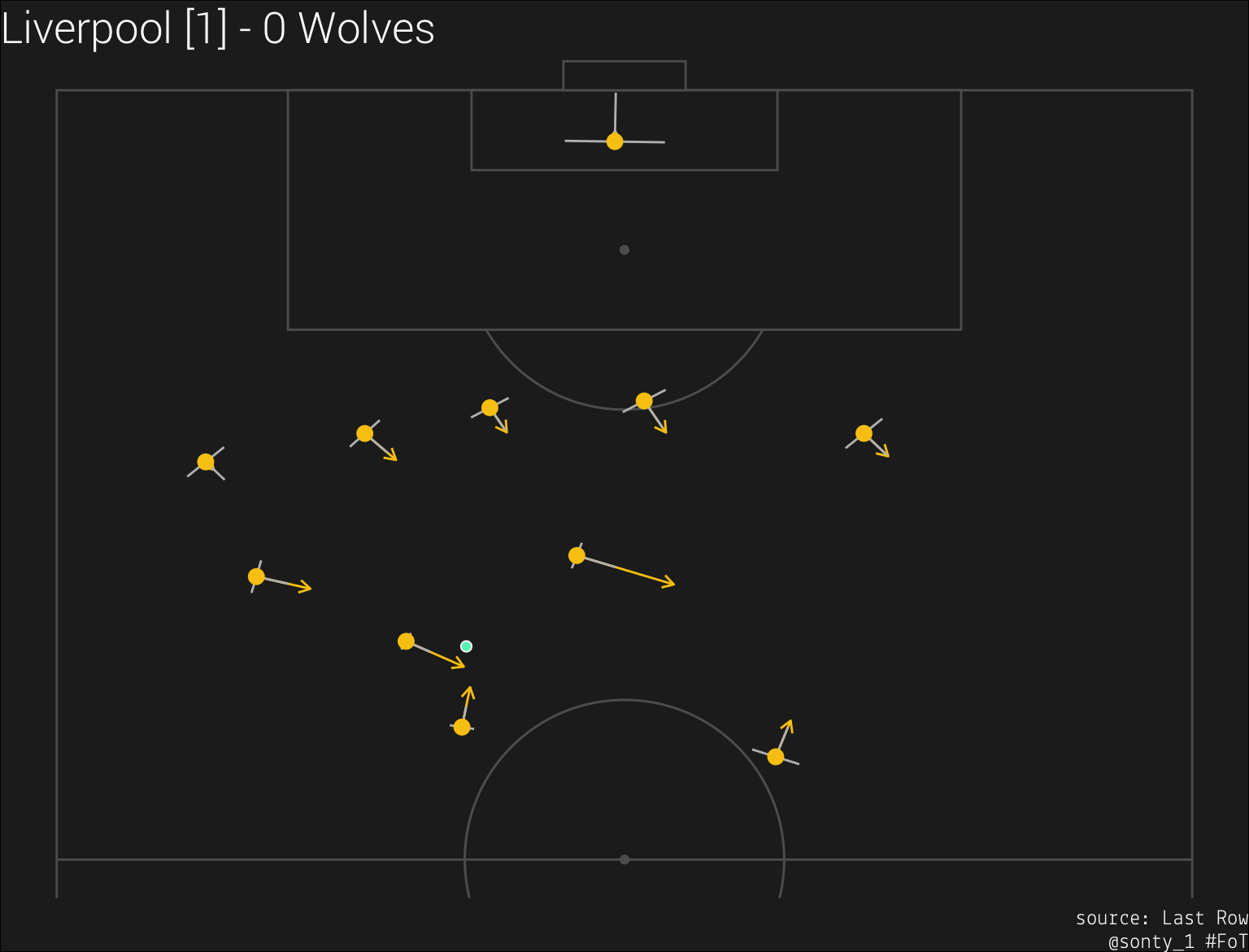 Note how the defenders’ obstruction radii diminish the closer they are to the ball.
> step 2: identify defenders that obstruct the shooter’s view on goal
The next step is to determine when a defender is in position to obstruct the shooter’s view of the goal. I did this by using the point.in.polygon function from the sp library for R.
 We can see that there are two defenders obstructing Mane’s view of the goal in this frame.
> step 3: project defenders obstruction onto the goal
Now that we know the obstruction radii for the defenders who are blocking the shooter’s goal-view, we can project the obstruction to the goal line (by tracing a line from the shooter, through the defenders’ obstruction radii, to the goal line). Since we have two points (the coordinates for the shooter and the defender’s obstruction locus) and the pitch length (106 meters), we can simply use the point-slope form of a line: \[y_{goal} = \frac{y_{shooter} - y_{obstructor}}{x_{shooter}-x_{obstructor}}(x_{goal} - x_{obstructor}) + y_{obstructor}\]
> step 4: determine the amount of the goal that is “controlled” by the shooter
Finally, we can use the obstruction projections to determine the amount of the goal line that is “controlled” by the shooter. I denoted goal control with \(\Gamma\) and defined the defense’s goal control as: \[\Gamma_{defense} := \frac{goalWidth - netGoalDistanceControlledByDefense}{goalWidth}\]. Hence, the shooter’s goal control is defined as: \[\Gamma_{shooter} := 1 - \Gamma_{defense}\] Note that a goal control value will always be in \([0, 1]\).
I’d like to offer a sincere thank you to the Friends of Tracking and the Seattle Sounders FC Analytics Department for all of the work they’ve been doing to make soccer analytics more accessible.
All code for this project can be found here (I’ll clean it up, I promise).