The Value of Pass Rush vs. Pass Protection
intro
With the 2020 NFL Draft looming, and all signs pointing to the Redskins drafting Chase Young with the 2nd overall pick, I wanted to do a quick analysis of the impact of a quality pass rush vs. quality pass protection. To do so, I’ll be using some of the NFL’s Next Gen Stats.
setup
Our dataset consists of stats for the top 4 pass rushers on each team in every game of the 2019 NFL regular season, here’s a quick sample:
pr %>%
  select(gameDate, week, team, opp, playerName, position, blitzCount, avgSeparationToQb) %>%
  sample_n(10) %>%
  arrange(gameDate) %>%
  head(10)
## # A tibble: 10 x 8
## gameDate week team opp playerName position blitzCount avgSeparationTo…
## <chr> <dbl> <chr> <chr> <chr> <chr> <dbl> <dbl>
## 1 09/22/20… 3 SEA NO Rasheem Gre… DE 11 3.68
## 2 09/29/20… 4 NO DAL Sheldon Ran… DT 19 4.79
## 3 10/13/20… 6 LAC PIT Isaac Roche… DE 9 4.25
## 4 10/20/20… 7 TEN LAC Harold Land… OLB 34 4.33
## 5 11/17/20… 11 BUF MIA Jerry Hughes DE 32 3.24
## 6 11/24/20… 12 NO CAR Sheldon Ran… DT 16 5.59
## 7 11/24/20… 12 NYG CHI Markus Gold… OLB 26 4.69
## 8 12/08/20… 14 TB IND Shaquil Bar… OLB 24 4.38
## 9 12/29/20… 17 JAX IND Calais Camp… DE 14 4.09
## 10 12/29/20… 17 DAL WAS Kerry Hyder DE 19 4.46The main stat we’ll be using is avgSeparationToQb.
data exploration
First, let’s get a general idea of the distribution of our data.
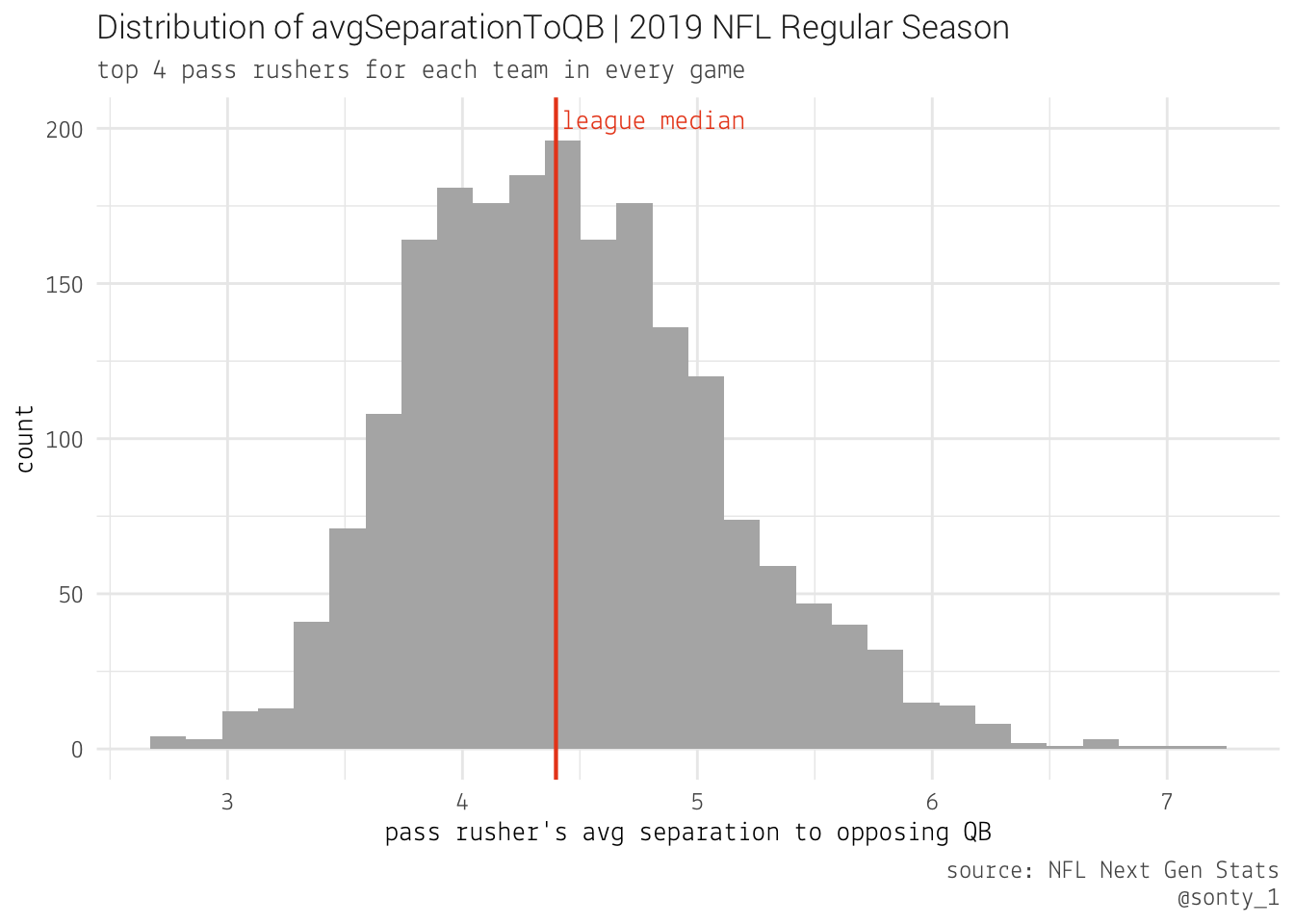
Since the distribution displays some skew, we’ll use the median as our measure of center. Let’s take a look at some of our top performers:
pr %>%
  select(week, team, opp, playerName, position, avgSeparationToQb) %>%
  arrange((avgSeparationToQb)) %>%
  head(20)
## # A tibble: 20 x 6
## week team opp playerName position avgSeparationToQb
## <dbl> <chr> <chr> <chr> <chr> <dbl>
## 1 10 LA PIT Aaron Donald DT 2.74
## 2 11 CLE PIT Myles Garrett DE 2.75
## 3 10 IND MIA Justin Houston DE 2.81
## 4 10 DAL MIN Robert Quinn DE 2.82
## 5 16 GB MIN Za'Darius Smith OLB 2.84
## 6 8 WAS MIN Matthew Ioannidis DE 2.87
## 7 12 ATL TB Adrian Clayborn DE 2.91
## 8 13 GB NYG Kyler Fackrell OLB 3.00
## 9 17 ATL TB John Cominsky DE 3.00
## 10 9 DAL NYG Michael Bennett DE 3.03
## 11 11 DEN MIN Shelby Harris NT 3.03
## 12 1 OAK DEN Arden Key DE 3.04
## 13 3 TB NYG Shaquil Barrett OLB 3.06
## 14 3 DAL MIA Robert Quinn DE 3.07
## 15 15 HOU TEN Charles Omenihu DE 3.08
## 16 8 ATL SEA Vic Beasley OLB 3.08
## 17 7 CIN JAX Geno Atkins DT 3.08
## 18 11 CAR ATL Gerald McCoy DT 3.10
## 19 17 PHI NYG Vinny Curry DE 3.11
## 20 8 CLE NE Myles Garrett DE 3.13Most of these players are the usual suspects. What sticks out to me is that, of the top 20 performances, 4 occurred against Minnesota and 4 occurred against the New York Giants.
Now, let’s take a look at pass rush distributions by team:
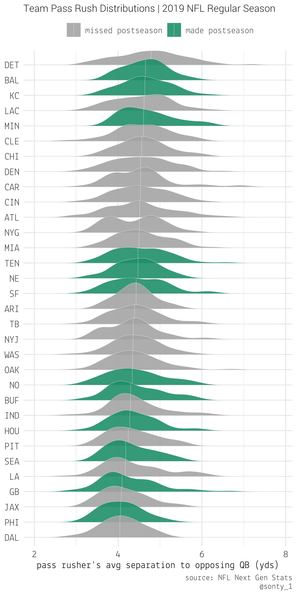
It appears as though teams with a lower median avgSeparationToQb have a better chance of making the postseason, but those clusters at the middle and top of the chart are interesting.
But pass rush is only one part of the battle in the trenches – what about pass protection? Well, by shifting our perspective, we can use the same avgSeparationToQb metric to get an idea of how teams’ offensive lines rank. Let’s take a look at the distributions for a team’s opposing pass rushers’ avgSeparationToQb.
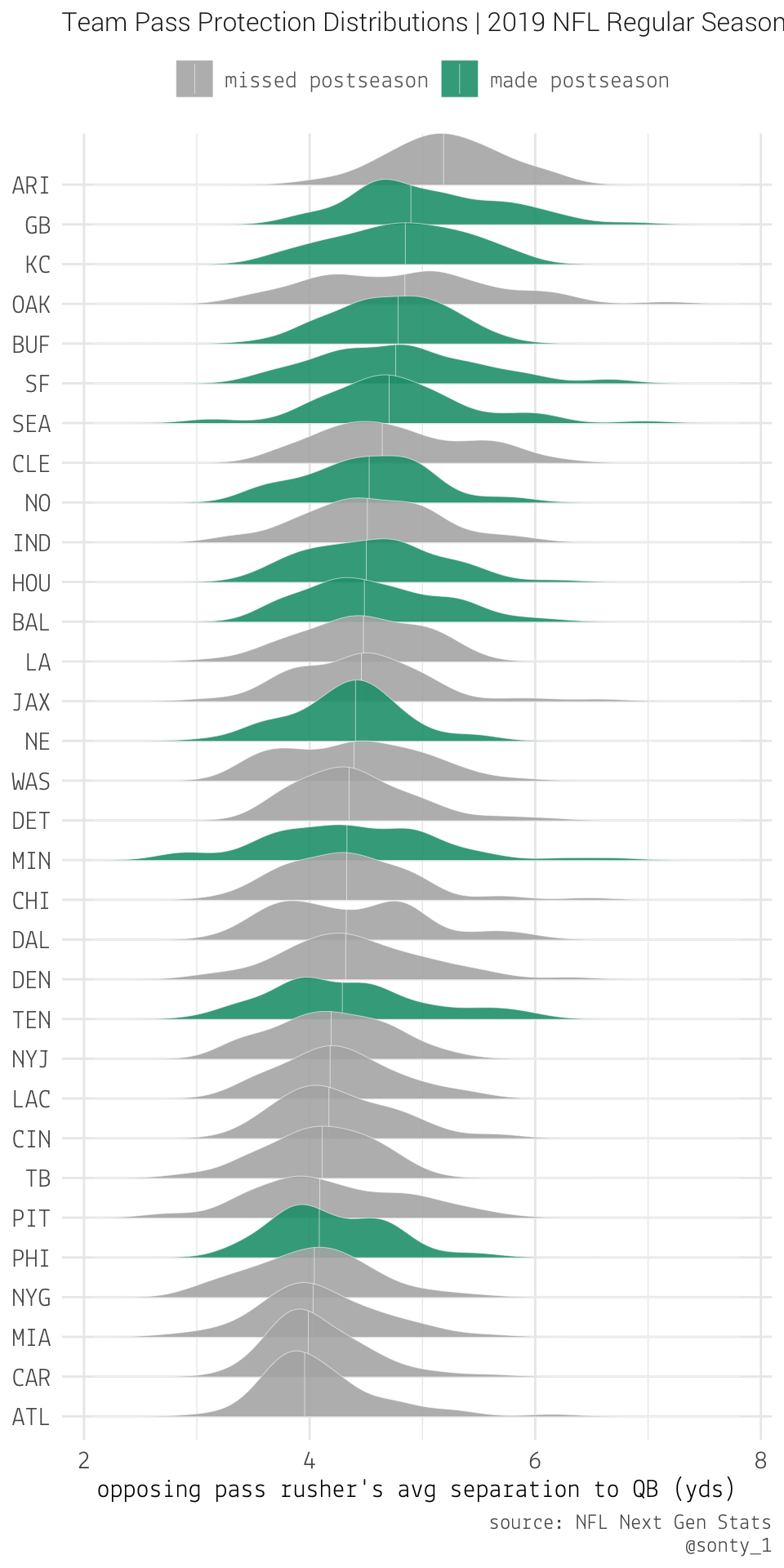
There appears to be a clearer trend here – teams who, on average, create more separation between their QB and the opposition’s pass rushers have a higher likelihood of making the postseason.
adjusting for opponent strength
Since we’ve got metrics for both pass rush and pass protection, we can use them to adjust team performances based on the strength of their opponents.
First, we’ll create point summaries for avgSeparationToQb per team. From the former ridgeline plots, we can see that team distributions are usually skewed, and in some cases even bimodal, so we’ll use the median here again (the median also helps correct for things like pass rushers being double-teamed, leading to them having high avgSeparationToQb numbers).
team_pass_rush <- pr %>%
  group_by(team, opp) %>% #gameId
  summarise(
    pr_game_med = median(avgSeparationToQb)
  ) %>%
  group_by(team) %>%
  summarise(
    team_expected_pr = median(pr_game_med)
  ) %>%
  arrange(team_expected_pr)
## `summarise()` regrouping output by 'team' (override with `.groups` argument)## `summarise()` ungrouping output (override with `.groups` argument)team_pass_pro <- pr %>%
group_by(team, opp) %>% #gameId
summarise(
pp_game_med = median(avgSeparationToQb)
) %>%
group_by(opp) %>%
summarise(
team_expected_pp = median(pp_game_med)
) %>%
arrange(desc(team_expected_pp)) %>%
rename("team" = "opp")## `summarise()` regrouping output by 'team' (override with `.groups` argument)
## `summarise()` ungrouping output (override with `.groups` argument)team_pass_rush %>% head(10)## # A tibble: 10 x 2
## team team_expected_pr
## <chr> <dbl>
## 1 GB 4.08
## 2 JAX 4.09
## 3 LA 4.12
## 4 DAL 4.13
## 5 PHI 4.16
## 6 SEA 4.21
## 7 BUF 4.21
## 8 TB 4.29
## 9 SF 4.31
## 10 HOU 4.32team_pass_pro %>% head(10)## # A tibble: 10 x 2
## team team_expected_pp
## <chr> <dbl>
## 1 ARI 5.10
## 2 GB 4.90
## 3 SF 4.81
## 4 OAK 4.80
## 5 KC 4.79
## 6 SEA 4.72
## 7 CLE 4.71
## 8 BUF 4.68
## 9 WAS 4.61
## 10 HOU 4.61We now have “expected values” for pass rush and pass protection for every team, we can use these to quantify the quality of a team’s performance against a certain opponent.
team_game_w_pass_rush <- pr %>%
  group_by(team, opp) %>%
  summarise(
    pr_game_med = median(avgSeparationToQb)
  ) %>%
  left_join(
    team_pass_pro,
    by = c("opp" = "team")
  ) %>%
  rename(
    opp_expected_pp = team_expected_pp
  ) %>%
  mutate(
    pr_diff = pr_game_med - opp_expected_pp
  )
## `summarise()` regrouping output by 'team' (override with `.groups` argument)team_game_w_pass_pro <- pr %>%
group_by(team, opp) %>%
summarise(
pp_game_med = median(avgSeparationToQb)
) %>%
left_join(
team_pass_rush,
by = c("team" = "team")
) %>%
rename(
opp_expected_pr = team_expected_pr
) %>%
mutate(
pp_diff = pp_game_med - opp_expected_pr
) %>%
rename(opp = team, team = opp)## `summarise()` regrouping output by 'team' (override with `.groups` argument)team_game_w_pass_rush %>% head(10)## # A tibble: 10 x 5
## # Groups: team [1]
## team opp pr_game_med opp_expected_pp pr_diff
## <chr> <chr> <dbl> <dbl> <dbl>
## 1 ARI ATL 4.33 3.95 0.380
## 2 ARI BAL 4.54 4.54 0
## 3 ARI CAR 3.97 4.02 -0.0455
## 4 ARI CIN 4.07 4.21 -0.144
## 5 ARI CLE 4.54 4.71 -0.171
## 6 ARI DET 4.36 4.36 0
## 7 ARI LA 4.73 4.61 0.122
## 8 ARI NO 4.42 4.48 -0.0539
## 9 ARI NYG 4.03 4.03 0
## 10 ARI PIT 4.58 4.12 0.470team_game_w_pass_pro %>% head(10)## # A tibble: 10 x 5
## # Groups: opp [1]
## opp team pp_game_med opp_expected_pr pp_diff
## <chr> <chr> <dbl> <dbl> <dbl>
## 1 ARI ATL 4.33 4.36 -0.0317
## 2 ARI BAL 4.54 4.36 0.181
## 3 ARI CAR 3.97 4.36 -0.386
## 4 ARI CIN 4.07 4.36 -0.292
## 5 ARI CLE 4.54 4.36 0.175
## 6 ARI DET 4.36 4.36 0
## 7 ARI LA 4.73 4.36 0.368
## 8 ARI NO 4.42 4.36 0.0622
## 9 ARI NYG 4.03 4.36 -0.331
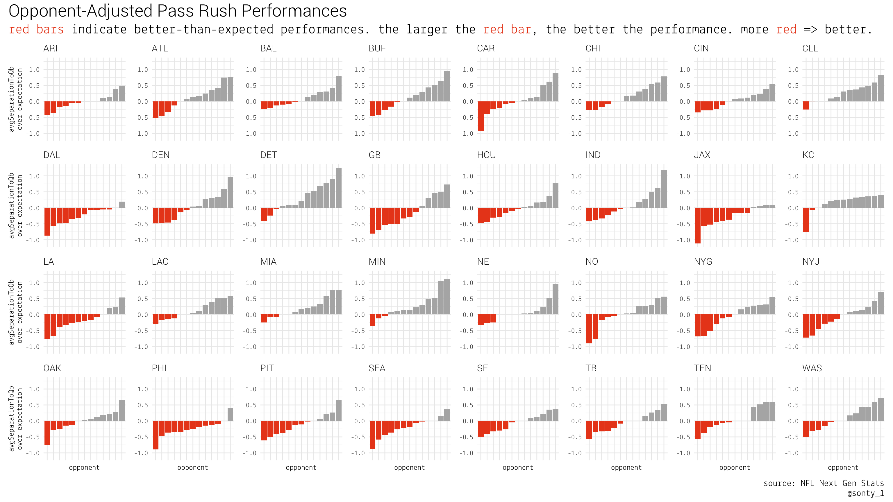
## 10 ARI PIT 4.58 4.36 0.225Let’s take a look at the opponent-adjusted pass rush performances. Since we defined these as \((medianAvgSeparationToQb) - (opponentExpectedAvgSeparationToQb)\), more negative values are better. You can interpret the following plot by looking at a team’s red bars, which represent better-than-expected pass rush performances. A larger red bar indicates a better performance.
We can create the same type of chart for opponent-adjusted pass protection performances In this chart, positive values are better, so superior teams will have more/taller blue columns.
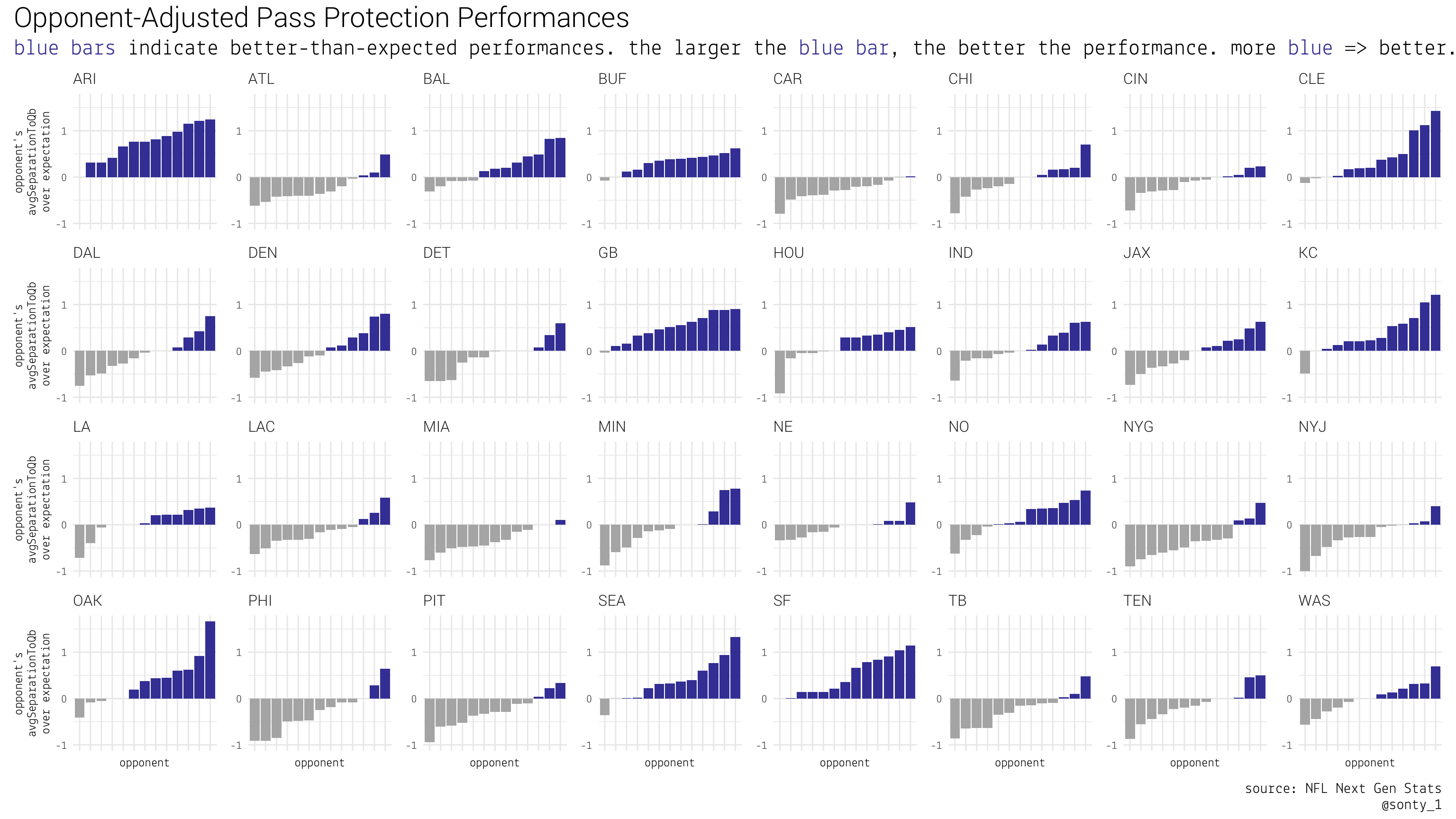
It looks like this metric is confounded by having a “mobile QB” (Kyler Murray is shifty), I think this highlights the value in having a QB that can pick up yards on the ground.
putting it all together
Finally, we can create point summaries for teams’ opponent-adjusted pass rush and pass protection perfomances (by summing teams scores and normalizing) and compare them to get an idea of how pass rush and pass protection impact a team’s chances of making the postseason.
pr_summ <- team_game_w_pass_rush %>%
  group_by(team) %>%
  summarise(
    team_w_pr_score = sum(pr_diff)
  )

pp_summ <- team_game_w_pass_pro %>%
  group_by(team) %>%
  summarise(
    team_w_pp_score = sum(pp_diff)
  )

final_summ_num <- pr_summ %>%
  left_join(pp_summ) %>%
  left_join(teams) %>%
  mutate(
    pr_score = 1-(team_w_pr_score-min(pr_summ$team_w_pr_score)) / (max(pr_summ$team_w_pr_score)-min(pr_summ$team_w_pr_score)),
    pp_score = (team_w_pp_score-min(pp_summ$team_w_pp_score)) / (max(pp_summ$team_w_pp_score)-min(pp_summ$team_w_pp_score))
  )

final_summ_num %>% select(team, pr_score, pp_score) %>% arrange(desc(pp_score))
## # A tibble: 32 x 3
## team pr_score pp_score
## <chr> <dbl> <dbl>
## 1 ARI 0.560 1
## 2 GB 0.755 0.785
## 3 SF 0.633 0.779
## 4 CLE 0.134 0.700
## 5 SEA 0.854 0.675
## 6 OAK 0.545 0.659
## 7 KC 0.289 0.659
## 8 BUF 0.324 0.615
## 9 BAL 0.370 0.514
## 10 NO 0.543 0.445
## # … with 22 more rows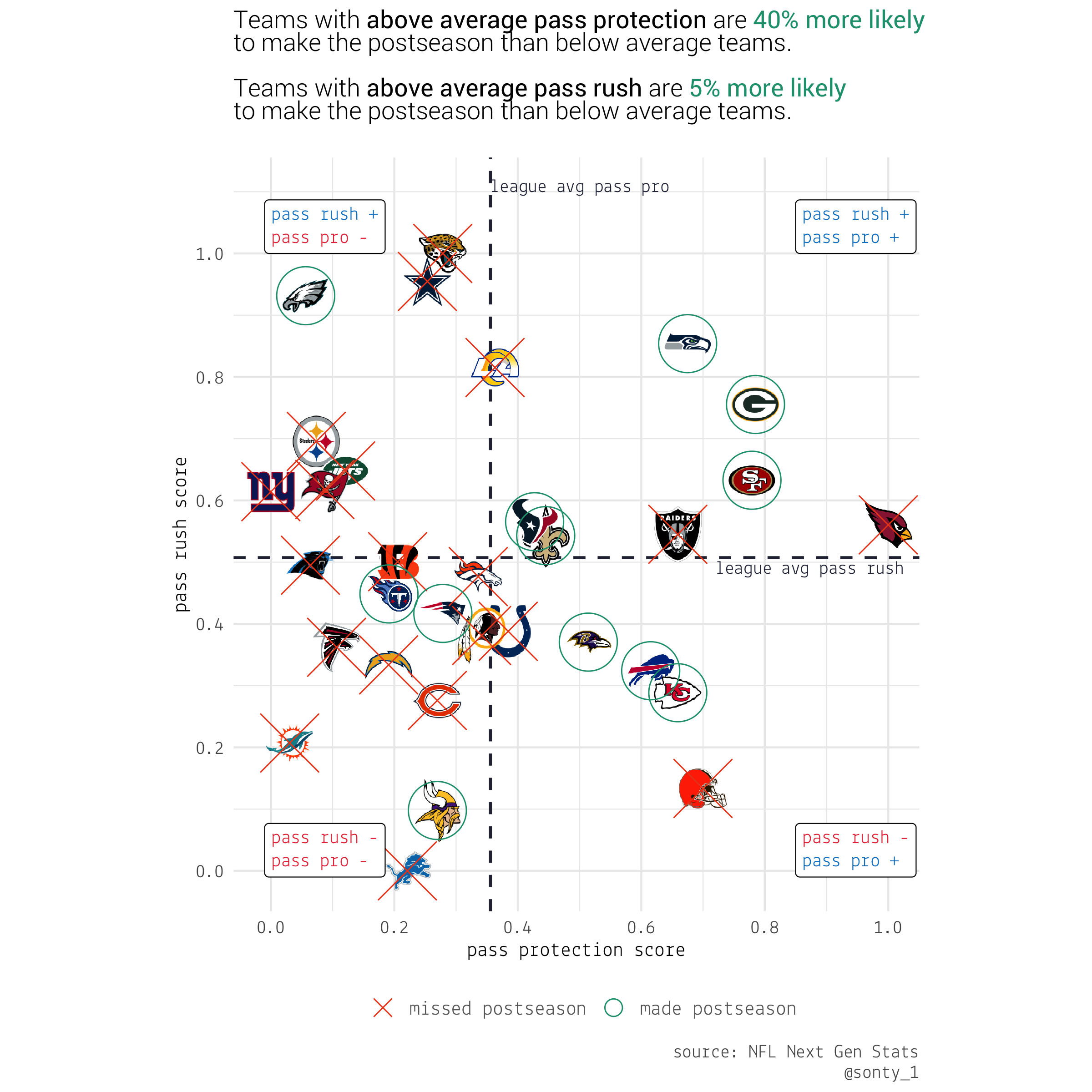
Observations from the chart:
- \(P[\mathrm{postseason} | \mathrm{aboveAvgPassRush}] = 6/15 = 0.40\)
- \(P[\mathrm{postseason} | \mathrm{aboveAvgPassProtection}] = 8/13 = 0.615\)
- \(P[\mathrm{postseason} | \mathrm{aboveAvgPassRush} \cap \mathrm{aboveAvgPassProtection}] = 5/8 = 0.625\)
- All 4 teams in the NFC West were above average in both pass rush and pass protection, that is a competitive division.
- GB was the only team in the NFC North that wasn’t below average in both pass rush and pass protection.
- All 4 NFC East teams had below average pass protection (by drafting Chase Young, the Redskins may be able to catch up to their division in pass rush score).
- NO was the only team in the NFC South with above average pass protection.
- BAL’s offseason signings indicate that they’re very aware of their below average pass rush.
- Outside of Kyler Murray (and his ability to scramble), no teams with rookie QBs had above average pass protection.
- TB already has an above average pass rush, it will be interesting to see how much impact Tom Brady’s knowledge of defenses will have on their pass protection score.
wrapping things up
From our analysis, it looks like the best path to the postseason is through better pass protection. avgSeparationToQb is a useful metric, but it appears to be quite confounded by mobile quarterbacks – it would be interesting to find a way to control for that in a new metric. It’s also important to note that this analysis makes no use of other valuable metrics like QB hurries, sacks, and QB knockdowns. In the future, I’d like to come back to these scores for pass rush and pass protection, and see how they correlate with opponent points scored and team points scored, respectively.